In this article, we are going to show you how to download historical stock prices using the Yahoo Finance API called « table.csv » and discuss the following topics that will allow you successfully import data in Excel from Yahoo in a simple and automatic way:

• Yahoo Finance API
• Import external data into Excel
• Import data automatically using VBA
• Dashboard and user inputs
• Conclusion

Before we delve into the details of this subject, we assume that you know how to program in VBA or, at least, that you have already some notions of programming, as we are not going to introduce any basic programming concepts in this article. However, we hope to post other articles in a near future about more simple aspects of programming in VBA.

You can find the whole code source of this tutorial on GitHub, or you can download the following Excel file that contains the VBA code together with the Dashboard and a list of stock symbols: yahoo-hist-stock.xlsm.

Yahoo Finance API

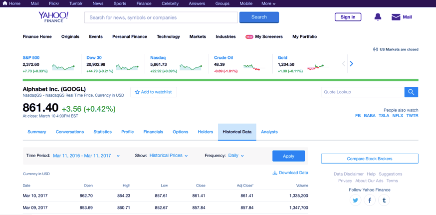
Yahoo has several online APIs (Application Programming Interface) that provides financial data related to quoted companies: Quotes and Currency Rates, Historical Quotes, Sectors, Industries, and Companies. VBA can be used to import data automatically into Excel files using these APIs. In this article, we use the API for Historical Quotes only.

It is of course possible to access Yahoo Finance’s historical stock data using a Web browser. For example, this is a link to access Apple’s historical data, where you can directly use the Web interface to display or hide stock prices and volumes.

Now, the first step before writing any line of code is to understand how the Yahoo Finance API for Historical Stock Data is working, which implies to first learn how URL (Uniform Resource Locator) are built and used to access content on the Web. A URL is a Web address that your browser uses to access a specific Web page. We give here some two examples of Yahoo’s URLs.

• This is how a URL look like when navigating on Yahoo Finance’s Web site:
  http://finance.yahoo.com/quote/GOOGL/history?ltr=1
• And this is how the URL of Yahoo Finance API look like when accessing historical stock data:
  http://ichart.finance.yahoo.com/table.csv?s=GOOGL&a=0&b=1&c=20 14&d=5&e=30&f=2016&g=d

Note that these URLs both access stock data related to symbol GOOGL, i.e. the stock symbol for Google.

However, except the fact that there are tow distinct URLs, they are also quite different in the result they return. If you click on them, the first simply returns a Web page (as you would expect), while the second returns a CSV file called table.csv that can be saved on your computer. In our case, we are going to use the table.csv file.

Here is an example of data contained in this file. The table.csv file contains daily stock values of Google from the 24th to 30th December 2015.

As you can see, the returned CSV file always contains headers (column names) in the first line, columns are separated by comma, and each line contains measurements for a specific day. The number of lines contained in the file depends on the given parameters (start data, end date and frequency). However, the number of columns (7) will always be the same for this API.

The first column [Date] contains the date for every measurement. Columns 3 to 5 [Open,High,Low,Close] contains stock prices, where [Open] represents the recorded price when the market (here NasdaqGS) opened, [High] is the highest recorded price for a specific time interval (e.g. day), [Low] is the lowest price for a specific time interval, and [Close] is the price after the market closed. [Volume] represents the number of transactions executed during the given time interval (e.g. for a day, between market opening and closure). Finally, the [Adj Close] stands for « Adjusted Close Price » and represents the final price at the end of the day after the market closed. It may not necessary be equal to the [Close] price because of different business reasons. So, usually, we prefer to use the Adjusted Close Price instead of the Close Price.

Now, if you look more closely at URL, we can see that it is composed of two main parts (one fixed and one variable): (1) the Web site and file name [http://ichart.finance.yahoo.com/table.csv] that is fixed, and (2) the parameters that can be modified in order to get historical data from other companies and/or for different periods of time [s=GOOGL&a=0&b=1&c=20 14&d=5&e=30&f=2016&g=d]. These two parts are separated with a special character: the question mark [?].

Let’s take a closer look at the the URL parameters following the question mark. Parameter name and value must always be passed together and are separated by an equal sign “=“. For example, parameter name “s” with value “GOOGL” gives parameter “s=GOOGL” that is then attached to the URL just after the question mark “?” as follow:

http://ichart.finance.yahoo.com/table.csv?s=GOOGL

Note here that only parameter “s” is mandatory. This means that the above URL is valid and will download a file containing all historical stock data from Google (on a daily basis), i.e. since the company was first quoted on the stock exchange market. All other parameters are optional.

Additional parameters are separated with symbol “&” from each other. For example, if the next parameter is “g=d” (for daily report), the URL becomes:

http://ichart.finance.yahoo.com/table.csv?s=GOOGL&g=d

Note the difference between “g” and “d”, where “g” is the parameter name whereas “d” is the parameter value (meaning “daily”).  Note also that the order in which parameters are appended to the URL is NOT important: “s=GOOGL&g=d” is equivalent to “g=d&s=GOOGL”.

For the Stock Symbol parameter “s”, a list of symbols (called tickers) can be found here.

Additionally, one might also want to to target a specific period of time. Fortunately, the API also accept parameters that allows us to reduce or increase the time window by using more parameters. Here is an exhaustive list of all parameters from the Historical Stock API:

Parameter Name	Description	Parameter Values
s	Stock Symbol	Any valid ticker (e.g. GOOGL, APPL, FB, etc.)
a	Start Month	[0 – 11] (0=January, 1=February, …, 11=December)
b	Start Day	[1 – 31] (depending on start month)
c	Start Year	[0 – this year] (e.g. 2017)
d	End Month	[0 – 11] (0=January, 1=February, …, 11=December)
e	End Day	[1 – 31] (depending on end month)
f	End Year	[0 – this year]
g	Frequency	{d, w, m, v} (Daily, Weekly, Monthly, or Dividend respectively)

Again, only parameter “s” is mandatory. Omitting all other parameters gives you the whole historical data for the given stock.

In short, there are 4 things that you can pass to the API (using the above 8 parameters).

• company [s]
• starting date [a, b, c]
• end date [d, e, f]
• frequency [g]

As explained above, the parameter s can take any valid stock symbol.

Parameter “a” represents the starting month and can have values from 0 to 11, where 0 is January, 1 is February, 2 is March, … and 11 is December. (Yeah, this does not make sense!) Parameter “b” represents the starting day and accept values from 1 to 31 (but, of course, this depends on the given month as not all months have 31 days). Parameter “c” represents the starting year. Parameters “d”, “e”, “f” represent the ending month, day and year, respectively, which have the same constraints as parameters “a” “b” and “c”. Finally, parameter “g” represents the data frequency and can take 4 distinct values: “d” for daily, “w” for weekly, “m” for monthly and “v” for yearly.

Hence, using all the above parameters can give, for example, the following URL:

http://ichart.finance.yahoo.com/table.csv?s=GOOGL&a=0&b=1&c=20 14&d=5&e=30&f=2016&g=d

Try to modify, add and remove the different parameters and their value to get a better understanding on how the Yahoo Finance API behaves.

Importing external data in Excel

Excel offers you several ways of importing external data into worksheets. You can import data from the following data sources: text files, Web pages, Access, SQL Server, or any another SQL database. Here, we are only going to deal with text files (such as CSV) and tables displayed on Web pages.

Import from Text Files

First, we show you how to import a CSV file stored locally on your computer into Excel. This part is crucial, as this will allow you to import and format CSV files automatically in a very simple and efficient way.

Start by downloading the table.csv file manually using this link: http://ichart.finance.yahoo.com/table.csv?s=GOOGL
(If this does not work, you can download the file directly from here: table.csv)

If you open the above file directly using Excel, chances are that (depending on your regional settings) that the file won’t be formatted as a regular table, but rather as a list of lines separated by comma. If your Windows is using US reginal settings, the CSV file will normally be formatted just fine. However, if you live in France, the CSV file will probably not be interpreted correctly. This is because in most (if not all) countries in Europe, the semi-colon is used as separator, whereas in the comma is used as separator.

Note: the difference in regional settings between countries (including but not limited to list separator, date and time) is actually the source of many bugs in software systems.

For this reason, you need to import the content of the CSV file into Excel using the “Text Import Wizard”, which will allow you to properly interpret the CSV format. To do so, open Excel and create a new Workbook. Then, click on the “Data” tab and select « From Text » in the “Get External Data” group. Locate and select the table.csv file and click OK. You should now be prompted with the “Text Import Wizard” window.

In Step 1, chose “Delimited”, as the different column in the file are delimited using a special character, namely the comma. Do not forget to precise that your file has headers (i.e. columns names) contained in the first line. Click Next.

In Step 2, you have to choose the delimiter that separate columns. Select “Comma” and deselect “Tab”. Leave the text qualifier as double-quote and click next.

In Step 3, leave all field formats to “General” and click Finish. Optionally, you can select “Date” as data format for the first column and choose YMD (Year-Month-Day) as date type, but dates will be formatted correctly even if you leave the format to “General”.

Finally, select the sheet and range where you want the data to be imported. The selected cell represents the upper-right corner of the new table containing the CSV data. Click OK.

You should obtain the following result:

Import from Web pages

Another way to import data into Excel is to import data directly from a table displayed on a Web page. The main difference from importing data from Text File is that the source and format is quite different from a text file. In fact, in this case, we the source is expected to be an HTML table (with tag <table>). Any other tag will not be considered. So, this means that if your data is not contained inside a table, you cannot (easily) import the data into Excel.

For instance, let’s assume that we want to import some data contained in the following Web page:

http://finance.yahoo.com/q/hp?s=GOOGL

To do so, you need to use the “New Web Query” wizard, which will allow you import a Web table into Excel. To do so, open Excel and create a new Workbook. Then, click on the “Data” tab and select « From Web » in the “Get External Data” group. Copy the above URL in to “Address” text box and click on the “Go” button. If you want other stock data, you can type http://finance.yahoo.com/, look for a specific stock symbol and click on “Historical Prices” menu item.

Note that Excel is using a legacy browser to access Web pages and you might be prompt with the following error multiple times:

Simply ignore this kind of errors by clicking Yes (or No) each time this pop-up window appears.

When this is over, you can finally select the table of interest as follow and click “Import”.

Note that it is possible to select and thus import several tables at once. If you want, you can also modify the “Set Date Range” parameters to obtain specific historical data for the current stock. In the example above, we selected weekly stock values from the 1^st of January to 14^th of March 2017, which gives the following URL:

http://finance.yahoo.com/q/hp?s=GOOGL&a=00&b=1&c=2017&d=02&e=14&f=2017&g=w

Note here that the resulting URL parameters are then same as the Yahoo Finance API (as explained in the previous chapters).

Finally, choose the target range where you want the Web table to be imported and click “OK”.

You should obtain the following result:

Congratulation, you now know how to import external data to Excel!

Import data automatically using VBA

We are going to show you how to automatically import historical stock data directly using Yahoo Finance API, but without having to download the file locally before importing it (as shown in the previous chapter).

The problem here is that we want to read data from an URL that returns a text file instead of a HTML page. However, if you try to access the Yahoo Finance API (e.g. http://ichart.finance.yahoo.com/table.csv?s=GOOGL) using the “New Web Query” wizard from Excel, a pop-up window will ask you to manually download the file locally. And of course, you cannot access online data source using the “Text Import Wizard”.

Fortunately, it is possible to use this API from Excel. However, for this purpose, we first need to better understand how Excel is working and, more precisely, what VBA code is generated when we import external data into Excel.

First you need to have access to and know how to record a macro in Excel.

One of the best feature of Excel is that you can generate VBA code based on your actions performed in Excel.  The Office Web site explain how you can generate a macro using Excel and how to display the “Developer” tab. Here we just gives a brief summary.

To generate a macro in Excel, click on the “Developer” tab and select “Record macro”.

Give a name to the macro you are going to generate and click OK (e.g. “LoadExternalData”).

Now, any action that you do in Excel will be recorded in this Macro (in a new module called Module1). And by “any action”, we mean that everything that you do will generate equivalent VBA code.

For instance, if now you click on cell B2 and write “Hello”, the following code will be generated:

Range(« B2 »).Select
ActiveCell.FormulaR1C1 = « Hello »

If later you decide to execute the macro again, all actions that you performed will be re-executed at once. Here, cell B2 will be selected and “Hello” will be written in B2.

As you might expect, Excel can do more than recording simple actions. In fact, Excel can also record more complex action such as importing external data. (Now you know where we am going!) The idea is to first start recording a macro and then import external data as shown in the previous chapter.

Hence, if you import the CSV file called table.csv from your computer, the following macro is generated:

Sub LoadExternalData()

    With ActiveSheet.QueryTables.Add(
            Connection:="TEXT C:\Users\julien.ribon\Desktop\table.csv ", _
            Destination:=Range("$A$1"))
        .CommandType = 0
        .Name = "table_1"
        .FieldNames = True
        .RowNumbers = False
        .FillAdjacentFormulas = False
        .PreserveFormatting = True
        .RefreshOnFileOpen = False
        .RefreshStyle = xlInsertDeleteCells
        .SavePassword = False
        .SaveData = True
        .AdjustColumnWidth = True
        .RefreshPeriod = 0
        .TextFilePromptOnRefresh = False
        .TextFilePlatform = 850
        .TextFileStartRow = 1
        .TextFileParseType = xlDelimited
        .TextFileTextQualifier = xlTextQualifierDoubleQuote
        .TextFileConsecutiveDelimiter = False
        .TextFileTabDelimiter = False
        .TextFileSemicolonDelimiter = False
        .TextFileCommaDelimiter = True
        .TextFileSpaceDelimiter = False
        .TextFileColumnDataTypes = Array(1, 1, 1, 1, 1, 1, 1)
        .TextFileTrailingMinusNumbers = True
        .Refresh BackgroundQuery:=False
    End With

End Sub

Note that if you are using Mac OSX, Excel will generate the following code, with the TextFilePlatform property set to xlMacintosh:

Sub LoadExternalData()

    With ActiveSheet.QueryTables.Add(
            Connection:="TEXT;Macintosh HD:Users:julien:Desktop:table.csv", _
            Destination:=Range("A1"))
        .Name = "table"
        .FieldNames = True
        .RowNumbers = False
        .FillAdjacentFormulas = False
        .RefreshOnFileOpen = False
        .BackgroundQuery = True
        .RefreshStyle = xlInsertDeleteCells
        .SavePassword = False
        .SaveData = True
        .AdjustColumnWidth = True
        .TextFilePromptOnRefresh = False
        .TextFilePlatform = xlMacintosh
        .TextFileStartRow = 1
        .TextFileParseType = xlDelimited
        .TextFileTextQualifier = xlTextQualifierDoubleQuote
        .TextFileConsecutiveDelimiter = False
        .TextFileTabDelimiter = False
        .TextFileSemicolonDelimiter = False
        .TextFileCommaDelimiter = True
        .TextFileSpaceDelimiter = False
        .TextFileColumnDataTypes = Array(1, 1, 1, 1, 1, 1, 1)
        .Refresh BackgroundQuery:=False
        .UseListObject = False
    End With

End Sub

On the other hand, if you import data from a Web page, the following macro is generated instead:

Sub LoadExternalData()

    With ActiveSheet.QueryTables.Add(
            Connection:= "URL;http://finance.yahoo.com/q/hp?s=GOOGL", _ 
            Destination:=Range("$A$1"))
        .CommandType = 0
        .Name = "hp?s=GOOGL"
        .FieldNames = True
        .RowNumbers = False
        .FillAdjacentFormulas = False
        .PreserveFormatting = True
        .RefreshOnFileOpen = False
        .BackgroundQuery = True
        .RefreshStyle = xlInsertDeleteCells
        .SavePassword = False
        .SaveData = True
        .AdjustColumnWidth = True
        .RefreshPeriod = 0
        .WebSelectionType = xlSpecifiedTables
        .WebFormatting = xlWebFormattingNone
        .WebTables = "15"
        .WebPreFormattedTextToColumns = True
        .WebConsecutiveDelimitersAsOne = True
        .WebSingleBlockTextImport = False
        .WebDisableDateRecognition = False
        .WebDisableRedirections = False
        .Refresh BackgroundQuery:=False
    End With
    
End Sub

When you are done, finish recording by clicking on “Stop recording” in the “Developer” tab.

Note that if you try to re-execute either of these macros, you will get the following error:

To solve this problem, remove the following line and your Macro should work like a charm.

.CommandType = 0

Now, let’s compare these two macros to illustrate both their similarities and differences.

As you can see, both macro are using an essential object to import external data, namely the QueryTable object. You can think of this object as containing a Query that produces a Table once executed.

Here is the official definition: the QueryTable object “represents a worksheet table built from data returned from an external data source, such as an SQL server or a Microsoft Access database” (or in our case Web pages and text files).

To create and execute a QueryTable, you need to first provide three things:

• a Worksheet that holds the QueryTable (e.g. Sheet1),
• a destination cell (e.g. $A$1) that holds the received data, and
• a connection string that contains the type of data source and its location in form of a URL.

Depending on the method chosen to import data, that connection string can be quite different. In our case, we have the following connections.

• From Text: « TEXT; C:\Users\julien.ribon\Desktop\table.csv »
• From Web: « URL;http://finance.yahoo.com/q/hp?s=GOOGL »

The rest of the Macro is actually composed of parameters that configures the QueryTable object to obtain the appropriate behavior. There are two groups of parameters: general parameters shared by both Macros and specific parameters that are related to the data source (i.e. Web vs. Text).

We are not going to explain every parameters here (you can read the official documentation to this purpose), but only the most important ones.

General parameters shared by both macros:

.Name = "table"
.FieldNames = True
.RowNumbers = False
.FillAdjacentFormulas = False
.PreserveFormatting = True
.RefreshOnFileOpen = False
.RefreshStyle = xlInsertDeleteCells
.SavePassword = False
.SaveData = True
.AdjustColumnWidth = True
.RefreshPeriod = 0
...
.Refresh BackgroundQuery:=False

RefreshStyle property tells how the data should be written into the given Excel sheet. Should the new table override exiting data or should it be inserted? xlInsertDeleteCells tells Excel in shift existing column to the right before importing new data. Instead, you should use xlOverwriteCells in order to override cells containing data. 

Refresh is not a property but a method: it execute the query and start importing the data in your Excel sheet. If you omit this line, nothing will happen. Additionally, this method can take an optional parameter called BackgroundQuery. This tells Excel if the query should execute synchronously or asynchronously. Meaning that the user either have to wait for data to arrive (BackgroundQuery:=False) or if it can continue to work without the data (BackgroundQuery:=True).

Specific parameters for Text files:

.TextFilePromptOnRefresh = False
.TextFilePlatform = 850
.TextFileStartRow = 1
.TextFileParseType = xlDelimited
.TextFileTextQualifier = xlTextQualifierDoubleQuote
.TextFileConsecutiveDelimiter = False
.TextFileTabDelimiter = False
.TextFileSemicolonDelimiter = False
.TextFileCommaDelimiter = True
.TextFileSpaceDelimiter = False
.TextFileColumnDataTypes = Array(1, 1, 1, 1, 1, 1, 1)
.TextFileTrailingMinusNumbers = True

These parameters all start with “TextFile” and represent the different option that you can choose in the “Text File Wizard” (as explained above).

TextFileParseType indicates whether the fields in your text files are delimited by specific characters such as commas or tabs (xlDelimited), or if columns are delimited by specific width (xlFixedWidth).  In our case, the CSV file is delimited by characters.

TextFileCommaDelimiter indicates that the CSV file is (or not) delimited by commas.

TextFileTextQualifier designates the type of text qualifier, i.e. the character that indicates the starting and ending point of a text. In our case, we let the default value (xlTextQualifierDoubleQuote), i.e. double quote (« ).

Specific parameters for Web pages:

.WebSelectionType = xlSpecifiedTables
.WebFormatting = xlWebFormattingNone
.WebTables = "15"
.WebPreFormattedTextToColumns = True
.WebConsecutiveDelimitersAsOne = True
.WebSingleBlockTextImport = False
.WebDisableDateRecognition = False
.WebDisableRedirections = False

These parameters are not important for the remaining of our task. However, the WebTables property is an essential parameter to import data from Web pages, as it indicates which tables that appear on the Web page should be imported. In this case, table number 15 is imported, but it is possible to import more than one table at once. For example, writing « 6,9,13,15 » will import the 6^th , 9^th 13^th and 15^th table displayed on the Web page.

The key idea is then to set up a QueryTable objet for a text file (as this corresponds to the returned data), while uing the address of the Yahoo Finance API in the connection string. The resulting connection string is therefore as follow:

« TEXT; http://ichart.finance.yahoo.com/table.csv?s=GOOGL »

And these are parameters (with their values) that should be used to configure and correctly import the data from the received CSV file:

Property	Value	Description
RefreshStyle	xlOverwriteCells	Replace cell values
BackgroundQuery	False	Synchronous query (wait for response)
TextFileParseType	xlDelimited	Separate columns with a character
TextFileTextQualifier	xlTextQualifierDoubleQuote	Value Delimiter = double-quote (”)
TextFileCommaDelimiter	True	Column Separator = comma (,)

Now, using the above connection string and parameters, we can build a macro that is able to automatically download historical data from Yahoo Finance:

Sub LoadExternalData()
    Dim url As String
    url = "TEXT;http://ichart.finance.yahoo.com/table.csv?s=GOOGL"
    
    With ActiveSheet.QueryTables.Add(url, Range("$A$1"))
        .RefreshStyle = xlOverwriteCells
        .BackgroundQuery = False
        .TextFileParseType = xlDelimited
        .TextFileTextQualifier = xlTextQualifierDoubleQuote
        .TextFileCommaDelimiter = True
        .Refresh ' run query and download data
    End With
End Sub

Not only is this solution elegant, it is also very efficient! In fact, we do not need to parse or format the using a (slow) loop, as this is directly done by the QueryTable object.

Voilà! You have successfully imported external data from one of Yahoo Finance APIs using Excel and VBA.

Now, the last step is to provide a dashboard in Excel so that users can directly interact with Yahoo Finance, without having to work with VBA.

Dashboard and user inputs

In this last chapter we are going to build an interface in Excel so that users can directly interact with the worksheet without having to modify VBA macros. We are therefore going to:

• read user input from specific Excel cells,
• transform these inputs into values in order to build a correct URL for Yahoo Finance,
• download the appropriate historical data based on the URL.

First, let’s build a simple interface. Start by defining cells that will holds user inputs and cells that will holds the downloaded data. This can, for example, look like the following worksheet:

Base on the above worksheet, we can define the following cells:

• Cell B2 contains the stock symbol (or ticker),
• Cell B3 contains the starting date,
• Cell B4 contains the ending date,
• Cell B5 contains the frequency, and
• Cell D1 will hold the external data.

Warning: you should NOT create or insert any table in columns D to J, because this will prevent the creation of QueryTable as we will see in the next section.

Now, it is important to properly define user inputs in order to avoid errors. To this extent, we can use “Data Validation” to limit the values that the user can enter. Select cell B2, Click on the “Data” tab and select “Data Validation” in the “Data Tools” group.

Now, select “List” under “Allow”, as we want to provide a whole list of stock symbols. Uncheck “Ignore blank” as the symbol is mandatory.

Under “Source”, you should select a list of existing symbols: the simplest approach is to store an exhaustive list of symbols in another worksheet. This list can be downloaded here.

For both B3 and B4, you should define a “Data Validation” that correspond to a date, where date in B3 (starting date) cannot be higher than B4 (ending date).

This is the data validation for B3:

And this is the data validation for B4:

Finally, you should also limit the number of values that users can enter in cell B5 (Frequency), where cell can only be one of the following value: Daily (d), Weekly (w), Monthly (m), and Dividend Only (v).

Again, this can be done using a data validation based on a list:

Finally, you can create a button called “Load” that will allow users to execute your macros and download the data from Yahoo Finance: on the “Developer” tab, click on “Insert” and then select the “Button” under “Form Controls”.

Now, this is how your dashboard should look like:

The Dashboard is now ready! We just need to implement the macro that will read and transform user inputs.

Reading and transforming user inputs

Write a Macro Sheet that read user inputs (StockSymbol, Start Date, End Date and Frequency) and format them so that they will be compatible with the URL of Yahoo Finance.

First, if are using data validation with a correct list of stock symbol, then there is nothing to be done for cell B2 (as the symbol can directly passed as such in the URL).

Now for dates, this is another story. In fact, you should split dates into three parts, namely day, month, and year, because each date is represented by three URL parameters. To extract each part, you can use the VBA functions called Day, Month, and Year, respectively. This is an example that illustrate how to extract these values out of the starting date:

Dim startDate As Date
Dim startDay As Integer , startMonth As Integer, startYear As Integer
    
startDate = Range("B3").Value
startDay = Day(startDate)
startMonth = Month(startDate) - 1
startYear = Year(startDate)

Warning: since URL parameters for months accept value between 0 and 11, you have to subtract 1 from the extracted month.

Finally, frequency should be mapped from the given values (e.g. “Daily”) to the appropriate symbol (e.g. “d”). This can easily be done using a condition, as follow:

Dim frequency As String
frequency = Range("B5").Value

Select Case frequency
Case "Daily"
    frequency = "d"
Case "Weekly"
    frequency = "w"
Case "Monthly"
    frequency = "m"
Case "Dividends Only"
    frequency = "v"
Case Else
    frequency = "" ' unknown frequency
End Select

Of course, you might want to directly use symbols d, w, m and v as list values in data validation so that you do not need to map values using VBA as explained above.

Note also that you might want to test if user inputs are empty, as only the stock symbol in mandatory for Yahoo Finance API.

Building the URL:

Now, it is time to build the URL for the QueryTable objet. The following macro builds and concatenates the different part of the URL string for Yahoo Finance:

Dim url As String
url = "http://ichart.finance.yahoo.com/table.csv"

' Add to the URL parameters based on the extracted values.
url = url & "?s=" & stockSymbol
url = url & "&a=" & startMonth
url = url & "&b=" & startDay
url = url & "&c=" & startYear
url = url & "&d=" & endMonth
url = url & "&e=" & endDay
url = url & "&f=" & endYear
url = url & "&g=" & frequency

Now, you just have to pass the resulting URL variable into the QueryTable Object as follow.

ActiveSheet.QueryTables.Add(url, Range("$A$1"))

Note that you might want to change the destination sheet and range according to your need.

Finally, depending on size of external data, i.e. the number of rows in the table, you prbably want to completely clear the range containing data before importing new data. This can easily be done with the following code (assuming that cell A1 is contained inside the data table):

Range("A1").CurrentRegion.ClearContents

This removes the whole table (but keeps the format) and thus avoids old data from the previous import to still be present in the worksheet.

Conclusion

Voilà! This concludes this article about importing Yahoo’s historical stock data using Excel and VBA. If you click on the “Load” button of the dashboard, you should obtain the following result:

You can find the whole code source of this tutorial on GitHub, or you can download the following Excel file that contains the VBA code together with the Dashboard and a list of stock symbols: yahoo-hist-stock.xlsm.

Please, feel free to write any comment about this article. We are looking forward to your feedback.

References

• QueryTable documentation
• Use Yahoo Finance as data source
• A List of All Yahoo Finance Stock Tickers
• Yahoo Finance – Historical Data (Web)
• Yahoo Finance – Historical Data (API)
• Google Code – Yahoo Finance Managed